May 8, 2024 Update: Interact with the machine learning (ML) version (version R2V4) of the new Fire Spread Model.
Project Goals
A major challenge for wildfire modelling is the ability to span the range of scales of fire phenomena. Fuel particle heat transfer and ignition occur over millimeters but wildfires impact landscapes and communities across kilometers. Even if the fine-scale physical processes of fire spread were well known, it is impractical to resolve them computationally for large domains of real fires. Thus, physics-based modelling has been much slower than real time and has not yet become operational for wildfire management. Even for research purposes on relatively small fires (~100 m2) using supercomputing clusters, physical models employing computational fluid dynamics in 3D must compromise spatial resolution to achieve performance and thus fidelity to the fine-scale fuel descriptions, and processes of heat transfer, ignition, and combustion.
An alternative approach to fire spread modelling is to limit the spatial domain to one-dimension (1D). A 1D formulation allows explicit resolving of the heat transfer and sequential ignition of discrete fuel particles at fine-scales and can be unambiguously compared with measured behaviors and capture the fuel heterogeneity. It solves a single 1D line spanning domains of about 50-200 m in less than a minute, but this is too slow to be implemented directly in simulations of large fires.
Google Research
Using the expertise and machine learning technology of Google Research, a deep learning (DL) approach was employed to represent the behavior of a high-resolution physics-based wildland fire spread model. The ultimate objective is being able to efficiently use the DL model for intensive simulations of large fires while retaining fidelity to the fine-scale physical processes. We begin with a fire model that reduces the spatial domain of the fire spread problem to one dimension (1D). The 1D model explicitly resolves cm-scale fuel variations, heat transfer and heating/drying dynamics of individual fuel particles and burning behavior of the bed. We then run the fire model 100’s of millions of times for factorial combinations of fuel, weather, and topographic conditions as training data for the DL algorithm. Rapid advances in the past decide in DL show it can represent complex and perhaps unknown relations among variables in the system.
One Dimensional Fire Spread Model
The dynamical nonlinear 1D fire spread model is explained in detail by Finney et al. (2021) and in a conference paper that overviews a more recent version (Forthofer et al., 2022). Briefly, the model domain is a 1D transect through a fuel bed with resolution nominally of 1 cm. At these resolutions, variations in fuel structure, such as gaps and clumps can be explicitly resolved in contrast to bulk fuel descriptions. Fire spread is an outcome of discrete particle ignition, which accelerates from the ignition state and achieves a steady rate of spread (ROS), flame length (FL), and flame zone depth (FZD).
To generate a dataset for training a DL model, the 1D fire spread model was run on factorial combinations of 13 input variables at 2cm resolution for a 100m fuel bed. For the initial demonstration, we chose only to represent steady state variables of fire spread rate, flame length, and flame zone depth from those data produced by the dynamical model. Others could include acceleration time and energy release from post-frontal combustion.
| Variable | Values | Units |
| Ignition depth | 0.1, 1.0, 2.0, 4.0 | m |
| Bed width | 1.0, 10.0, 20.0, 30.0, 40.0, 50.0 | m |
| Slope angle | 0.0, 10.0, 20.0, 30.0 | degrees |
| Wind type | steady, sine wave | m/s |
| Wind mean speed | 1.0, 2.0, 3.0, 4.0, 5.0, 6.0, 8.0, 10.0 | |
| Wind amplitude fraction of mean | 0.2, 0.4, 0.6, 0.8, 1.0 | |
| Wind period | 1.0, 3.0, 5.0 | s |
| Particle diameter | 0.001, 0.002, 0.003, 0.004, 0.005 | m |
| Particle moisture | 2.0, 4.0, 6.0, 8.0, 10.0, 12.0, 15.0, 25.0, 35. | percentage |
| Fuel loading | 0.05, 0.1, 0.2, 0.5, 0.825, 1.55, 2.275, 3.0 | Kg/m2 |
| Fuel depth | 0.1, 0.2, 0.3, 0.4, 0.5, 0.6, 0.8, 1.0 | m |
| Fuel clump size | 0.5, 1.0, 2.0 | m |
| Fuel gap size | 0.0, 0.1, 0.2, 0.3, 0.4, 0.5 | m |
Table 1. List of variables and input values for generating training data sets from the 1D physical fire model. Total combinations 637,009,920.
Pre-processing
The dataset is filtered to only keep data points where the 1D model reported realistic ROS values of no more than 10 m/s. The dataset is further normalized before model training such that all input variables are normalized into [0, 1] linearly between 0 and the max value of corresponding variable, and output variables are first square-rooted and then normalized in the same fashion as they're skewed and have a long tail. The dataset is randomly split into train (65%), validation (15%) and test datasets (20%) for model development before any filtering. The train dataset is used to learn the parameters of the DL model, while the validation dataset is used to select the best model to avoid overfitting the train dataset. The test dataset is never seen during model development and is reserved to measure the generalization quality of the DL model in the end.
Deep Learning Model
Google Research used a two staged approach for predicting the steady-state variables. First, they used a binary classification model that predicts whether there is any fire at all (meaning the fire does not spread under the given conditions). If there is a prediction of no fire, then the ROS, FL and FZD are all zero. Otherwise, the regression model is used to perform the final prediction. Given the relatively few inputs to the model, we chose the quintessential Feed-Forward Neural Network (FFNNs) for both models. More specifically, they used a fully connected FFNN, which allows for a rich latent space that grows exponentially with the number of input features. As such, it is not appropriate for domains with large numbers of input features, but often works surprisingly well for smaller domains. The DL models are trained on the training dataset such that the Mean Squared Error (MSE) (or binary cross-entropy, i.e., logistic loss) for the regression (or classification) model is minimized. L2 regularization was applied to avoid model overfitting. The learning rate and the learning rate decay rate were empirically determined by training multiple models and then selecting the models with the lowest loss on the validation dataset.
- The DL model captured the wildfire trends from the 1D model.
- Use of the detailed 1D fire model as part of a large-scale wildfire simulation (2D or 3D) would provide the correct physics on combustion and steady state statistics but is infeasible due to the computational cost. Therefore, the primary goal for the DL model is to approximate the 1D model as accurately as possible at a dramatically reduced computational cost. For comparison, the average 1D model run time for the training data set was about 70 s for each of 78,125 cases, whereas the DL model takes about 0.01 s for each case.
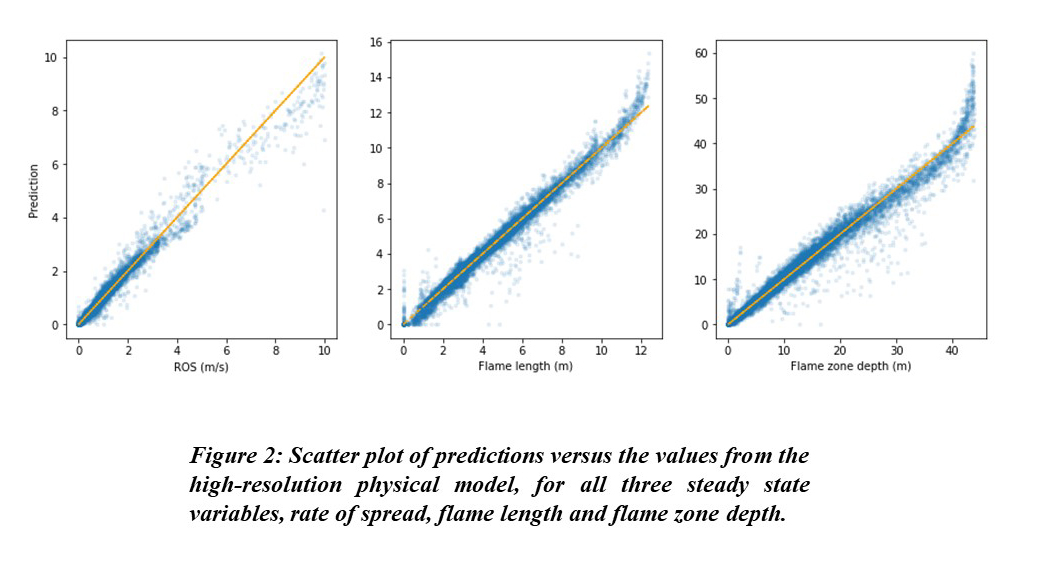
- Scatter plots of the predicted dependent variables versus those from the underlying physical model for the test dataset show that most of the data points are quite close to the perfect reference (y = x) line. The mean (standard deviation) of the absolute errors for the dependent variables of ROS, FL, and FZD are 0.078 (0.17) m/s, 0.21 (0.29) m and 0.98 (1.53) m, respectively. Those numbers are close to that for the validation dataset, demonstrating that the DL model is capable of accurately reproducing the fire model’s behaviour.
- The example fire characteristics represented by ROS, FL and FZD are key descriptors of frontal fire behavior. We found that errors made by the DL model are at the extremes of the input data. The error around zeros is an indicator that more work is required for the classification model in differentiating the no-fire cases correctly, which is an important problem in practical fire management. The overall underestimate for large ROSs and overestimate for large flames might be related to dataset filtering, as the wind speed is at most 5 m/s, while we keep ROSs up to 10 m/s for cases with combined wind and high slope angle.
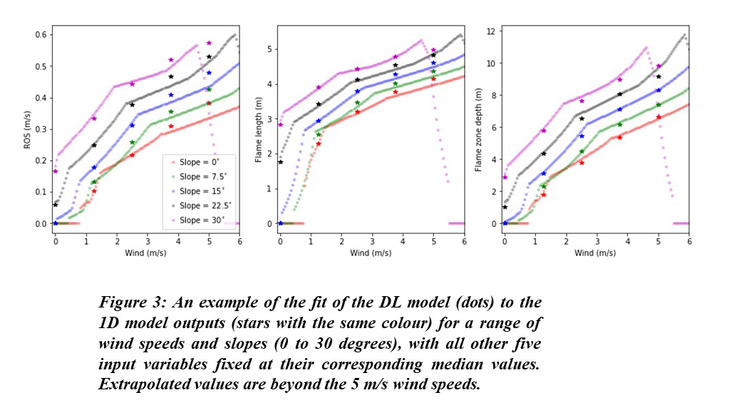
- The DL model captured the monotonic dependence of fire behavior on the wind speed and terrain. It also and illustrates some extrapolation beyond the training data since the whole dataset training data included only wind speeds up to 5 m/s, not only at the discrete wind speeds reported by the 1D model, but also over the continuous range. However, inevitably, at some point the models' limitations become apparent. Extending the models’ accuracy to higher wind speeds can potentially be resolved by including training data at higher wind speeds or considering a probabilistic DL model, both of which are subjects of ongoing work.
Future directions
- We are working to increase the size of the of training dataset. Once time-varying winds and heterogeneous fuel types are included, the number of training data could reach into the billions.
- We intend to host the training data openly for all machine learning researchers to access.
- Google Research and the USFS are aiming for a stand-alone DL surrogate of the fire model as a demonstration of its feasibility and utility
- We are envisioning a demonstration of the DL surrogate model as a substitution for the Rothermel fire spread equation in a 2D fire simulation model such as FARSITE.